IFCraft is a browser-based tool that generates IFC files from CAD geometry and alignment data. It is the reverse of a BIM checker: instead of reading and validating IFC, it writes IFC from native geometry you already have — from Rhino 3DM, DXF, DWG, GLB, OBJ, or LandXML alignments.
The tool runs entirely in your browser. There is no server; the model you open stays in browser memory on your machine and is never uploaded anywhere. This means you do not have to worry about sharing sensitive project data with a third party, and the tool works offline once you have the files. A Chromium-based browser (Chrome or Edge) is required — IFCraft uses the File System Access API for reading and saving files, which Firefox and Safari do not yet support.
The web application is available at ifcraft.checkthebim.com/app.
To follow along with this guide, a finished IFC from the demo project (the final state, including the georeferencing from chapter 11) is available for download: demo-bridge-so201.ifc
The central concept in IFCraft is the Convention. A Convention is a complete description of how your source data is assembled into an IFC file. It contains:
IfcProject through the site down to individual
elements),A Convention is saved as a portable .ifcb.json file. The
main value of this approach is reuse: define a Convention
once — for example as a company or sector standard for bridges
— and reuse it across projects. On a new project you
supply a different source file; the tree and rules carry over
unchanged.
IFCraft writes three IFC schemas. Which one to choose depends on what you need to deliver:
ReferenceView_V1.2.CoordinationView_V2.0.IfcBridge,
IfcRoad, IfcRailway, and linear placement
along an alignment axis. Mapped to ReferenceView or
Alignment-basedView when at least one linear placement is
present.Accepted input formats:
.3dm — Rhino (recommended source for
triangulated mesh geometry),.dxf — tessellated geometry (MESH /
3DFACE) as well as 3DSOLID bodies (ACIS data is
converted to meshes automatically, see chapter 4),.dwg — AutoCAD 2007–2018; layers,
groups, and 3DSOLID bodies — the conversion runs directly in your
browser,.glb and
.obj — mesh geometry,.xml in LandXML
format — horizontal and vertical alignments for linear infrastructure
projects.Multiple source files can be used in a single project (for example a 3DM geometry file plus a LandXML alignment file).
Work in IFCraft follows a fixed sequence of steps. The tabs at the top of the application correspond to this sequence:
The typical workflow is Start → Tree → Enrichment → IDS check → Generate. (In the top bar the tabs appear in the order Tree · IDS · Enrichment · Generate; this guide covers enrichment before IDS because the requirement check builds on the properties you fill in.)
.ifc file. See chapter 7.The top bar is the same on all screens after a project is open:
.ifcb.json; keyboard shortcut Ctrl+S),
language toggle CS / EN, and the theme button (switches
between light and dark mode). The ? button opens this
guide in a new tab without interrupting your work.Saving and opening files uses the browser's File System Access API. The first time you save, the browser asks you to choose a file location; subsequent saves write to the same file automatically.
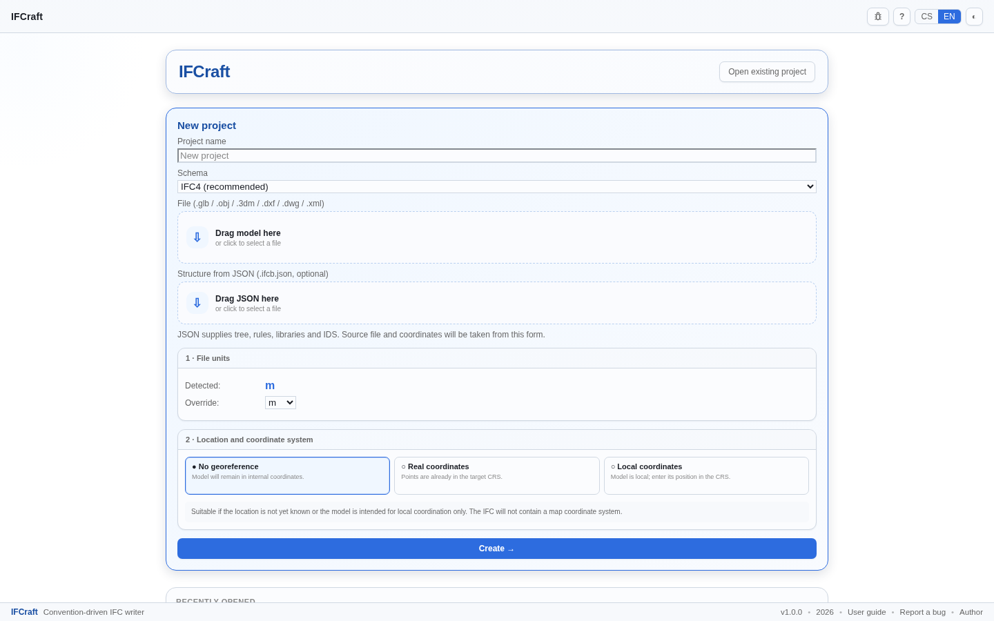
The start screen is the first thing you see when you open IFCraft. From here you create a new project or open a saved one.
Fill in the New project form from top to bottom:
Demo Bridge SO 201).IFC4 (recommended), IFC2x3 (legacy), and
IFC4x3 ADD2 (infra: bridges, roads, railways). See chapter
1 for an explanation of each schema.Bridge (IfcBridge), Road (IfcRoad),
Railway (IfcRailway),
Marine facility (IfcMarineFacility), or
General facility (IfcFacility). The default is Bridge.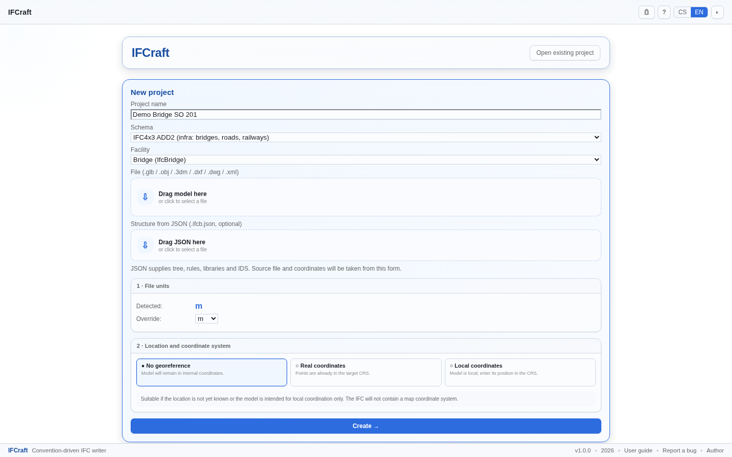
In this example the project is named Demo Bridge SO 201
with schema IFC4x3 ADD2 (infra: bridges, roads, railways)
and facility Bridge (IfcBridge). No source file has been
uploaded at this point — the drop zone is still empty.
Below the basic fields is the File (.glb / .obj / .3dm / .dxf
/ .dwg / .xml) area — the "Drag model here" drop zone. Drag a
source file with geometry or alignments here, or click to browse for a
file. Optionally, drag an existing .ifcb.json Convention
into the second drop zone ("Drag JSON here"); this carries over the
tree, rules, and libraries from that Convention, while the source file
and coordinate settings come from the current form.
The 1 · File units block shows two fields:
m). Important: this value is a static form
default, not a result of parsing the uploaded file. The
source file is not parsed until you press the Create
button. If you know your source data uses different units, change them
in Override: before clicking Create.m, cm, mm, in,
ft).The 2 · Location and coordinate system block offers three modes:
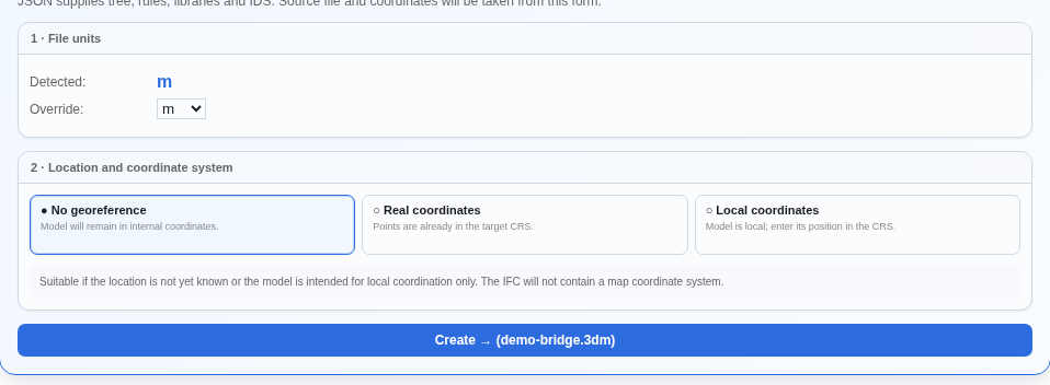
Georeference can also be changed later; chapter 11 covers it in detail.
The fastest way to get a complete tree is to use a saved Convention
as a template: drag a previously saved .ifcb.json file into
the Structure from JSON drop zone. The new project will
inherit the full tree, rules, and libraries (PSets, materials,
classifications) from that Convention — only the source file and
georeference settings are taken from the current form. You then re-bind
the layers of the new source file to the element slots in the Tree
editor (chapter 3). A Convention defined once can be reused for all
similar projects.
Without a template a minimal skeleton is created (IfcProject → Site → facility) and you build the tree manually in the Tree editor (chapter 3).
The button at the bottom of the form is labelled Create
→. When a source file is loaded it also shows the file name,
for example Create → (demo-bridge.3dm). Clicking it parses
the source file and creates the project.
After clicking Create, IFCraft parses the source
file and moves to the Tree view. The left-hand panel
shows the source file name and the number of layers it contains (for
example demo-bri… rhino3dm · 41 layers). The canvas shows
the initial spatial skeleton: IfcProject → Site → IfcBridge
(for an IFC4x3 bridge project).
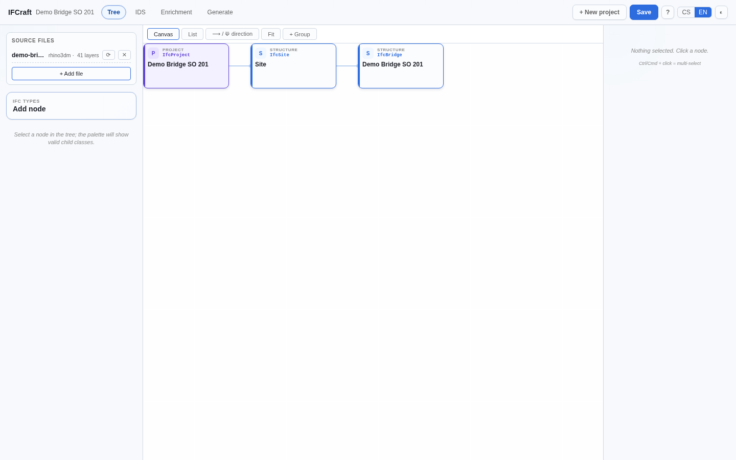
No layers are bound to element slots yet. The next step is to add element nodes under the bridge and bind layers to them — this is covered in chapter 3.
The Open existing project button in the top-right
area of the start screen loads a previously saved
.ifcb.json Convention. After opening or saving a project,
an entry appears in the RECENTLY OPENED list at the
bottom of the start screen. The list is populated by opening or saving
(not by mere creation) — IFCraft remembers the file via the browser's
File System Access API.
You can save at any time using the Save button in the top bar, or with the Ctrl+S shortcut. The first save prompts you to choose a file location; subsequent saves write to the same file without a dialog.
The Tree editor is the heart of IFCraft. This is
where you define the spatial and element structure of the future IFC
file — from the IfcProject root, through the site and the
facility, down to individual structural elements — and where you bind
source-file layers to those elements.
The centre of the screen shows the Canvas: a graphical view of the tree where each node is represented by a card. Spatial container nodes (project, site, bridge) appear on the left and branch rightward toward elements. On the left is the panel with Source files (chapter 4) and the palette for adding nodes; on the right is the detail panel for the selected node.
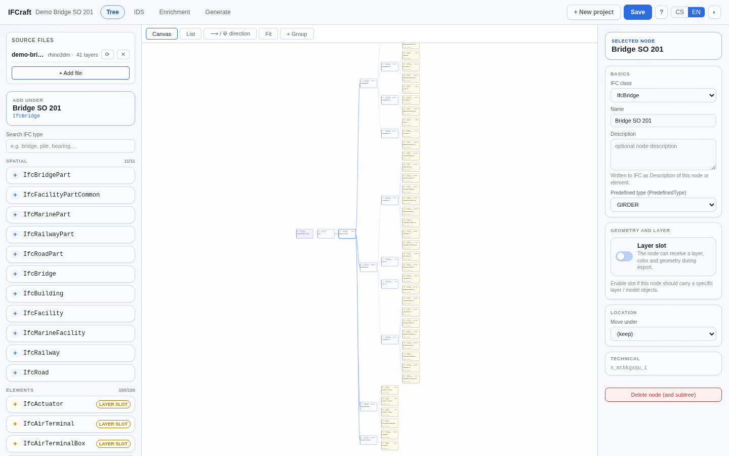
The toolbar above the canvas provides the following controls: Canvas / List (view toggle), ⟶ / ⟱ direction (switches between horizontal and vertical layout), Fit (zooms and pans so the whole tree is visible), and + Group (see below).
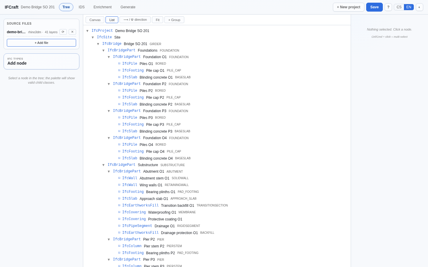
Click List to switch from the canvas to a row-by-row list, which is more readable for large trees. Each row shows the IFC class, the node name, the PredefinedType, and — where a rule binds one — the bound layer.
Every card on the canvas shows a type badge in the upper-right corner. There are two fundamentally different node types:
IfcProject, IfcSite, and infrastructure types
such as IfcBridge, IfcBridgePart,
IfcRoad, and IfcRailway. Structure nodes
organise the hierarchy; they carry no geometry themselves (with a narrow
exception for facility parts, discussed in chapter 5).IfcPile, IfcBeam, IfcSlab,
IfcFooting, and so on. Element nodes carry a LAYER
SLOT, which means they can receive geometry from a source-file
layer.Element nodes also show a LAYER indicator below the badge: either the name of the bound layer (when a layer has been assigned) or the word unbound (when no layer is assigned yet).
To add a node, first select a parent node by clicking its card, then choose a class from the palette on the left. The palette heading "ADD UNDER" shows the name and class of the current parent.
The key feature of the palette is that it does not offer arbitrary classes — it offers only those that are valid children of the selected parent according to the IFC composition rules. The palette divides the available classes into two sections:
11/11) shows how many classes are
available.A Search IFC type field at the top of the palette lets you filter classes by name.
In the example above, the selected node is IfcBridge, so
the SPATIAL section offers IfcBridgePart,
IfcFacilityPartCommon, IfcMarinePart, and
others — exactly the spatial classes that may appear directly under a
bridge.
For a typical multi-span bridge, a recommended practice is to use
IfcBridgePart nodes as named groups under
IfcBridge. Each support (abutment, pier) and each bridge
zone (substructure, superstructure, surface structure) gets its own
IfcBridgePart. This is not just organisational convenience
— it mirrors how BIM viewers (BIM Vision, Solibri, Navisworks) display
the model tree, makes quantities unambiguous per support, and allows
downstream coordination systems to filter by support number or zone.
In the Demo Bridge SO 201 example the tree is subdivided as follows:
Bridge SO 201 (IfcBridge, GIRDER) →
Foundations (IfcBridgePart, FOUNDATION) with four
sub-parts Foundation O1 / P2 / P3 / O4, each containing
Piles, Pile cap, and
Blinding concrete → Substructure
(IfcBridgePart, SUBSTRUCTURE) → Superstructure
(IfcBridgePart, SUPERSTRUCTURE) → Surface structure
(IfcBridgePart, SURFACESTRUCTURE).
Clicking a node opens its detail in the right-hand panel. The panel header shows "SELECTED NODE" with the node name. For element nodes it also shows the LAYER SLOT badge.
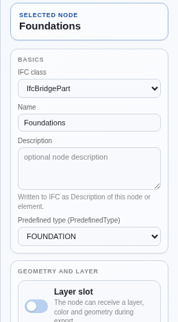
The BASICS section lets you edit:
Description.IfcElement.Tag (for example PIL-001). Visible
only on element nodes.IfcBridgePart the
available values include FOUNDATION,
SUBSTRUCTURE, SUPERSTRUCTURE,
SURFACESTRUCTURE, PIER, ABUTMENT,
and others. For IfcPile the options are BORED,
DRIVEN, COHESION, FRICTION,
etc.Setting the correct PredefinedType is important: IFC validation tools check that the value matches the entity class, and BIM viewers use it to label and colour elements automatically.
An element slot (LAYER SLOT) is the connection point between a tree node and source geometry. Each element node in the tree has a slot. In the GEOMETRY AND LAYER section of the node detail, the Layer slot toggle enables the slot. Once the slot is enabled, the Add layer field lists all layers from the source files loaded in the project — typing into the field filters the list (the search ignores accents), and the ⛶ (Open picker) button next to it opens a large search dialog, handy for files with dozens of layers. Selecting a layer binds it to the node; the slot changes from "unbound" to showing the bound layer name, and a BOUND LAYER block appears with the layer selection and colour settings.
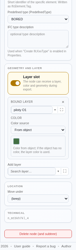
At export time, the geometry from the bound layer is used to create the IFC element's shape representation. A node without a bound layer produces an IFC element with no geometry.
When an element slot carries geometry, IFCraft can treat the objects in the bound layer in two ways (set in Enrichment → Properties, chapter 5):
Piles O1 contains multiple individual piles, and each pile
should appear as its own IfcPile in the IFC. The group key
is defined by how objects are grouped in the source file (Rhino groups,
GLB parents, or DXF ACAD_GROUP entities).Pile cap O1 that is
one continuous concrete volume regardless of how many mesh faces it
contains.Below the bound-layer selection the COLOR section has a Color source dropdown:
A colour preview swatch appears below the dropdown. For composite elements (chapter 8), each layer has its own color-source block.
To move a node to a different parent, use the Move under dropdown in the LOCATION section of the node detail. The dropdown lists all spatial containers that are valid parents for the node's class. Select the new parent and the node moves; the canvas redraws to reflect the new position.
Hold Ctrl (on macOS Cmd) and click additional nodes to select more than one at a time. The right panel shows a multi-select summary with the count and classes of selected nodes, and offers bulk actions such as deleting all selected nodes.
Independently of selection, nodes can be visually organised into canvas groups using the + Group button. A group dialog lets you give the group a name, description, and colour, and add nodes to it either from the current selection or one by one from a dropdown. Groups are a purely visual organising tool for the canvas — they are not written to IFC and do not create any rules or hierarchy.
A Convention does not have to rest on a single source file. IFCraft
can combine multiple sources in one project — typically a geometry file
from Rhino (.3dm) and horizontal/vertical alignments from
LandXML (.xml). Source files are managed in the panel on
the left side of the Tree editor.
The Source files panel is in the upper-left area of the Tree editor. Each file entry shows its name, type, and a brief statistic — for geometry files the number of layers, for LandXML the number of alignments. Next to each file are two buttons: ⟳ to replace the file and ✕ to remove it. At the bottom of the list is the + Add file button.
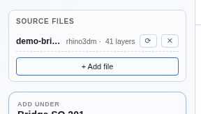
Click + Add file to add another source to the
Convention. The most common combination is a geometry file
(.3dm, .dxf, .dwg,
.obj, or .glb) plus alignments from a LandXML
file. After selecting a file an import modal appears
summarising what was loaded.
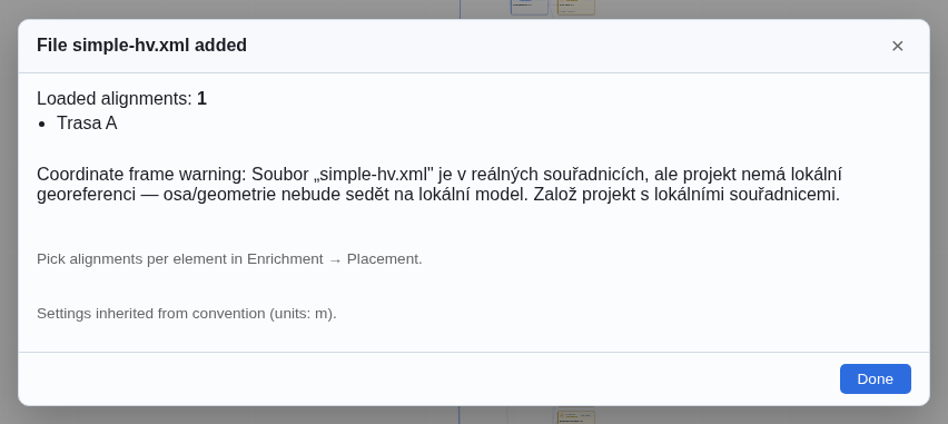
The modal confirms the file name and type. For LandXML it lists the loaded alignments (in the example: one alignment named Trasa A). If there is a mismatch between the file's coordinate frame and the project's frame, a warning is shown — for example when the LandXML is in real-world coordinates but the project has no georeference set, the alignment would lie hundreds of kilometres away from the local geometry. Resolve this either by founding the project with local georeference (chapter 11) or by using an alignment in the same coordinate frame as the model.
After confirming with Done the panel shows both files.
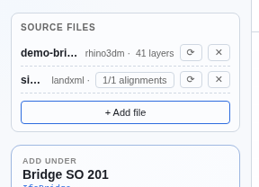
For a LandXML file the panel shows a 1/1 alignments button (or N/M where M is the total number of alignments in the file and N is the number of active ones). Clicking the button opens a picker where you enable or disable individual alignments. Alignments are then assigned to element slots in the Enrichment editor (chapter 10).
IFCraft also reads AutoCAD .dwg files
(versions 2007–2018). The conversion runs entirely in your browser — the
first DWG upload downloads a conversion module (about 3 MB) in the
background; the file itself never leaves your machine.
3DSOLID bodies from both DXF and DWG
are converted to meshes directly, without a CAD kernel: planar faces,
cylinders, spheres, tori and cones, and NURBS surfaces including trimmed
ones. After the file loads, the app summarises the result, for example
"3D solids (ACIS): 101/101 fully recovered".
The only solids that cannot be converted are those with no ACIS data
stored in the file, or those using exotic surface types. In that case
convert them to meshes in AutoCAD with the _MESHSMOOTH
command and save, or export .3dm instead.
Click ⟳ next to a file to replace it with a different version (for example, a newer revision of the geometry). After you select the replacement file IFCraft computes a layer diff: it compares the layers of the old and new files and shows which layers connected without changes, which are new, which disappeared, and which were renamed. Based on this diff it remaps rules so that element slots do not lose their geometry.
If all layers are present in the new file under the same names, no rules are affected and the modal reports zero changes. If layers are renamed or removed, the affected slots become unbound and must be re-bound manually. A Convention defined carefully for a project will survive routine geometry updates because the layer names are agreed in advance.
Click ✕ next to a file to remove it. Before the removal IFCraft performs an impact analysis and shows which rules would lose geometry and which elements would fall back from linear to absolute placement. Rules are preserved in the Convention even after removal: once the file is added again, all bindings are restored automatically. The dialog offers Remove anyway and Cancel buttons.
If no rules depend on the file (for example when removing a LandXML file that has not yet been assigned to any element), the analysis reports "No rules depend on this file" and removal is safe.
IFCraft always works in a single shared project coordinate frame. When you add a file that is in real-world coordinates, the tool automatically transforms (bakes) its geometry into the project's local frame so that geometry and alignments from different sources align with each other. How the result is exported back to a real-world CRS (for example for as-built delivery) is covered in chapter 11.
Once the tree stands and the element nodes have layers bound, enrichment begins. On the Enrichment tab you add everything that turns raw geometry into a real BIM model: geometry settings, non-graphical properties (PSets), materials, classifications, documents, and library references. All of this attaches to tree nodes — select a node on the left and work with its detail in the centre.
The Enrichment screen has three vertical panels. On the left is the Object tree — the same hierarchy as in the Tree editor, but presented as a flat, scrollable list. Each node shows its IFC class icon and counters for what is already attached: how many PSets, classifications, documents, or library references it has. The list header shows a summary line with the total number of slots and how many have properties.
In the centre is the detail of the selected node. The header shows "SELECTED NODE" with the node name, IFC class, and PredefinedType. Below it are two tabs: Node properties (geometry settings) and PSet (non-graphical). Click between them to switch.
On the right is a panel that switches between four editors: Material, Classification, Documents, and Libraries. The switch buttons are at the top of the panel.
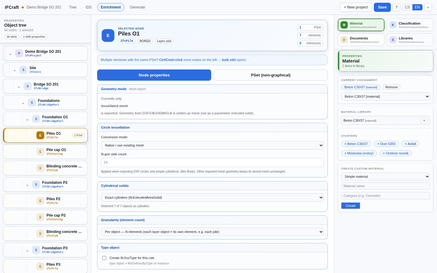
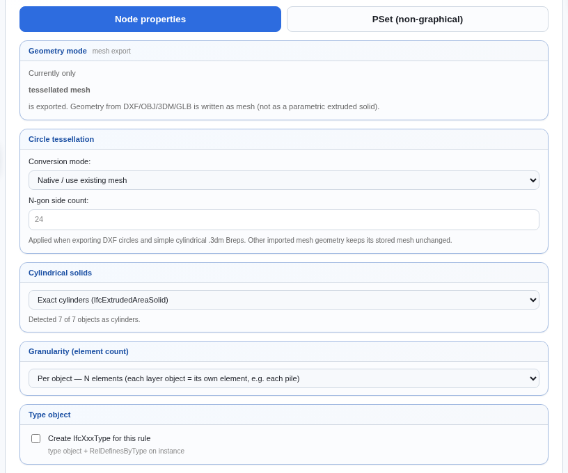
The Node properties tab controls how the bound geometry is turned into IFC. The cards shown depend on what the node contains — the set of cards differs between nodes.
Geometry mode. The first card is informational: it states that the current export mode is tessellated mesh — geometry from DXF, OBJ, 3DM, or GLB is written to IFC as a triangulated mesh, not as a parametric extruded solid.
Circle tessellation. Controls how circles and simple
cylinders are converted. The Conversion mode dropdown
has two choices: "Native / use existing mesh" (keeps the mesh exactly as
imported) and "Convert circle to n-gon". For the second choice you set
the N-gon side count (default 24). This setting applies
only when exporting DXF circles and simple cylindrical .3dm
Breps; other imported mesh geometry is kept unchanged.
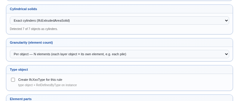
Cylindrical solids. This card appears only on nodes where IFCraft detects cylindrical objects. In the Demo Bridge project it appears on Piles O1 (IfcPile) — the seven bored piles on support O1 are detected as cylinders. The dropdown offers two options:
The label below the dropdown reports how many objects were detected as cylinders — in the demo "Detected 7 of 7 objects as cylinders".
Note on IFC4x3 and MVDs: for exact cylinders in IFC4x3, the official buildingSMART validator reports warning IFC430 — parametric solids such as
IfcExtrudedAreaSolidare outside the scope of the declared ReferenceView MVD. The file is valid and common viewers read it without issues; if you want a warning-free validator run, switch to Mesh (tessellation). The demo project therefore writes the piles as mesh in its final export — the downloadable demo IFC is stored that way too.
Granularity (element count). Decides how many separate IFC elements are created from one layer:
Type object. Ticking "Create IfcXxxType for this rule" tells IFCraft to generate a type object (for example IfcPileType) and link it to the instances via RelDefinesByType. A type object groups shared properties of multiple identical elements.
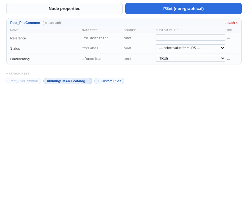
A Property Set (PSet) is a named group of non-graphical properties —
for example Pset_PileCommon with properties Reference,
Status, and LoadBearing. You can attach as many PSets as needed to each
node. Click the PSet (non-graphical) tab to switch.
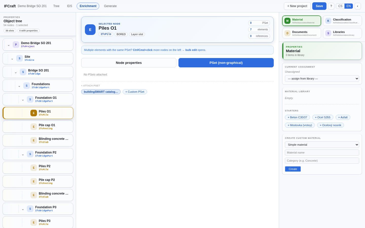
When a node has no PSets attached, the panel shows "No PSets attached." and an + ATTACH PSET section with two chips: buildingSMART catalog… and + Custom PSet. If you have previously created a custom PSet in the project, it also appears as a chip for quick re-attachment.
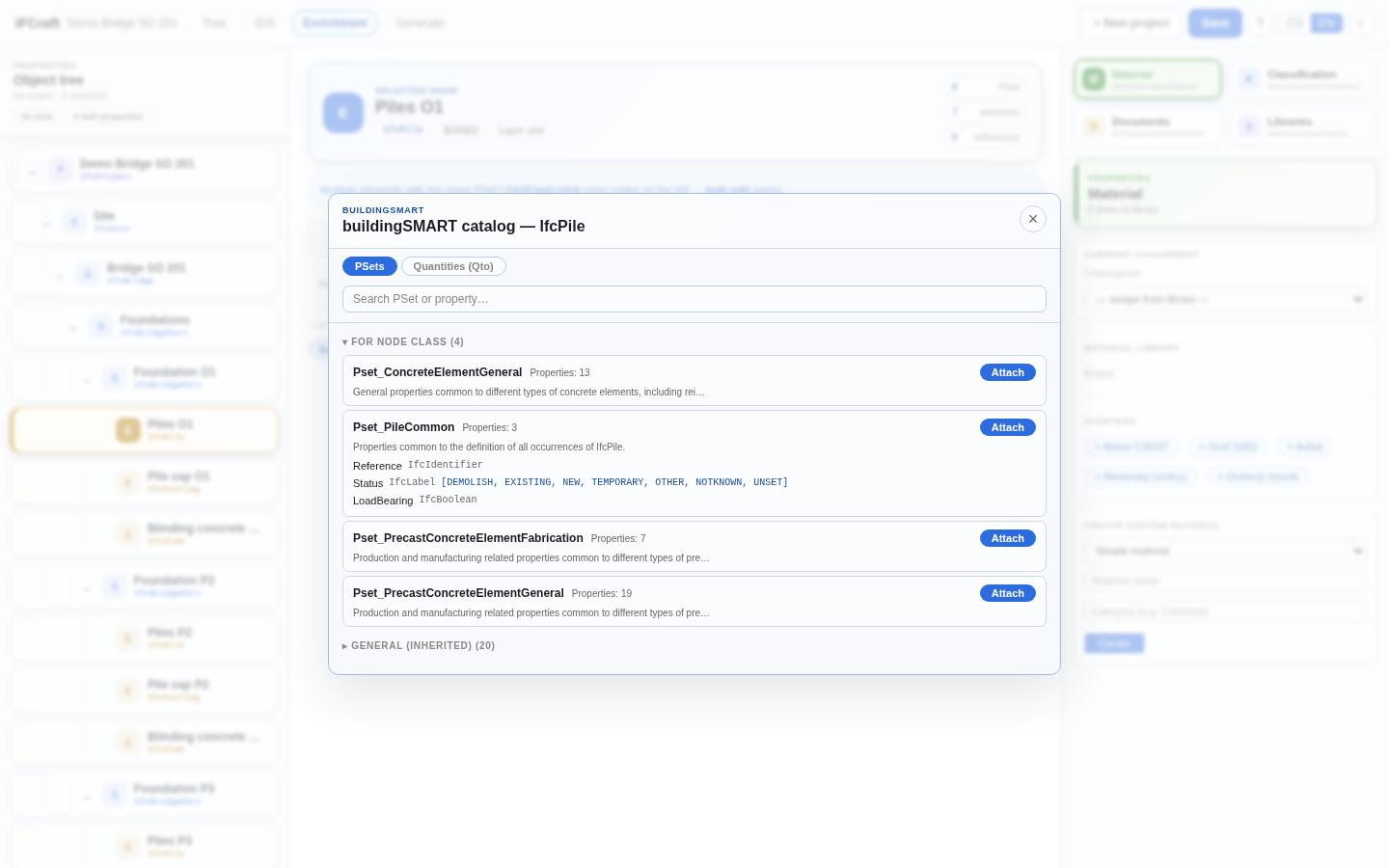
Clicking buildingSMART catalog… opens a modal with
the full set of PSets from the official IFC specification. The modal has
two tabs at the top: PSets and Quantities
(Qto). In the PSets tab, two sections are shown: FOR
NODE CLASS (PSets defined specifically for the element's IFC
class — for IfcPile these are Pset_PileCommon,
Pset_ConcreteElementGeneral, and others) and
GENERAL (INHERITED) (PSets applicable to any class;
collapsed by default). A search field filters by PSet name or property
name.
Each PSet in the catalog shows its name and the number of properties. Clicking the row expands it to show the list of properties with data types and IFC descriptions; enumeration properties also list the permitted values. Click Attach to attach the PSet to the node — the row switches to "attached". Closing the modal immediately shows the attached PSet in the panel.
In the table of an attached PSet, each row has columns
NAME, DATA TYPE,
SOURCE, CUSTOM VALUE, and
IDS. In the CUSTOM VALUE column you enter or override
the value for this element. Enumeration properties offer a dropdown with
the permitted values (for example, Status lists DEMOLISH,
EXISTING, NEW, TEMPORARY…). Only filled-in properties are
exported — empty properties are not written to IFC, and a PSet
with no filled properties is not created at all; a deliberately entered
empty string is written. An attached PSet can be
detached with the "detach ×" button in the PSet
header.
When a standard template is not enough, click + Custom
PSet. A form opens: enter a name (for example
Demo_Bridge_Properties), click + property
to add a row, name the property, and choose a data type (for example
IfcLabel or IfcReal). Click Create to attach the PSet
to the node.
The SOURCE column shows where a property value comes
from — typically const (a fixed value you enter). IFCraft
can also read values from native attributes of the
source geometry: Rhino UserStrings (custom object
attributes in .3dm files). In the custom PSet editor you
can set the source to "From model (UserString)" and
enter a key — the name of the attribute to read from
each object. When granularity is "Per object — N elements", each
resulting IFC element receives the value from its own object's
UserString (if the key exists on that object). If the key is missing,
the template default is used.
Priority of sources: manual override (CUSTOM VALUE) > UserString value (if key found on the object) > template default.
The catalog's Quantities (Qto) tab shows standard
Qto templates (for example Qto_PileBaseQuantities). Qto
sets hold numeric measurements — volumes, areas, lengths, counts — and
are written as IfcElementQuantity entities, separate from
IfcPropertySet. Quantities are available for IFC4 and
IFC4x3 schemas only.
Each quantity in an attached Qto template shows its source in the SOURCE column:
IFCraft computes Net quantities only (NetVolume, NetSurfaceArea, NetLength…). Gross quantities are not computed — enter them manually as overrides if needed. A Qto set with no values is not written to IFC.
The Color source setting for a node's bound layer lives in the Tree editor (GEOMETRY AND LAYER section, COLOR block). The four options are:
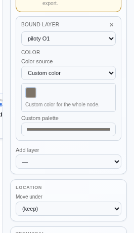
In the Demo Bridge project the starting convention uses From object for most elements (colours come from Rhino layer assignments in demo-bridge.3dm). Chapter 3 shows the colour source dropdown in context; refer to that chapter for the Tree editor detail panel layout.
When multiple nodes need the same PSet or value, Ctrl+click (macOS: Cmd+click) additional nodes in the left tree to enter bulk edit mode. The centre panel switches to "N selected nodes / SHARED PSETS" and shows only PSets that all selected nodes share. Editing the Common value column writes the value to all selected nodes at once. The + Add PSet to all selected button attaches a new PSet to the entire selection.
The right panel switches between four association editors. All four work with one selected node that has a bound layer.
Material. The Material panel assigns a material to the element. At the top is the current assignment dropdown ("— assign from library —"). Below it is the MATERIAL LIBRARY list and a STARTERS section with quick buttons (for example "+ Beton C30/37", "+ Ocel S355"). Clicking a starter adds the material to the library; then select it from the dropdown to assign it. The CREATE CUSTOM MATERIAL form supports three material kinds: Simple material, Layer set (IfcMaterialLayerSet), and Profile set (IfcMaterialProfileSet).
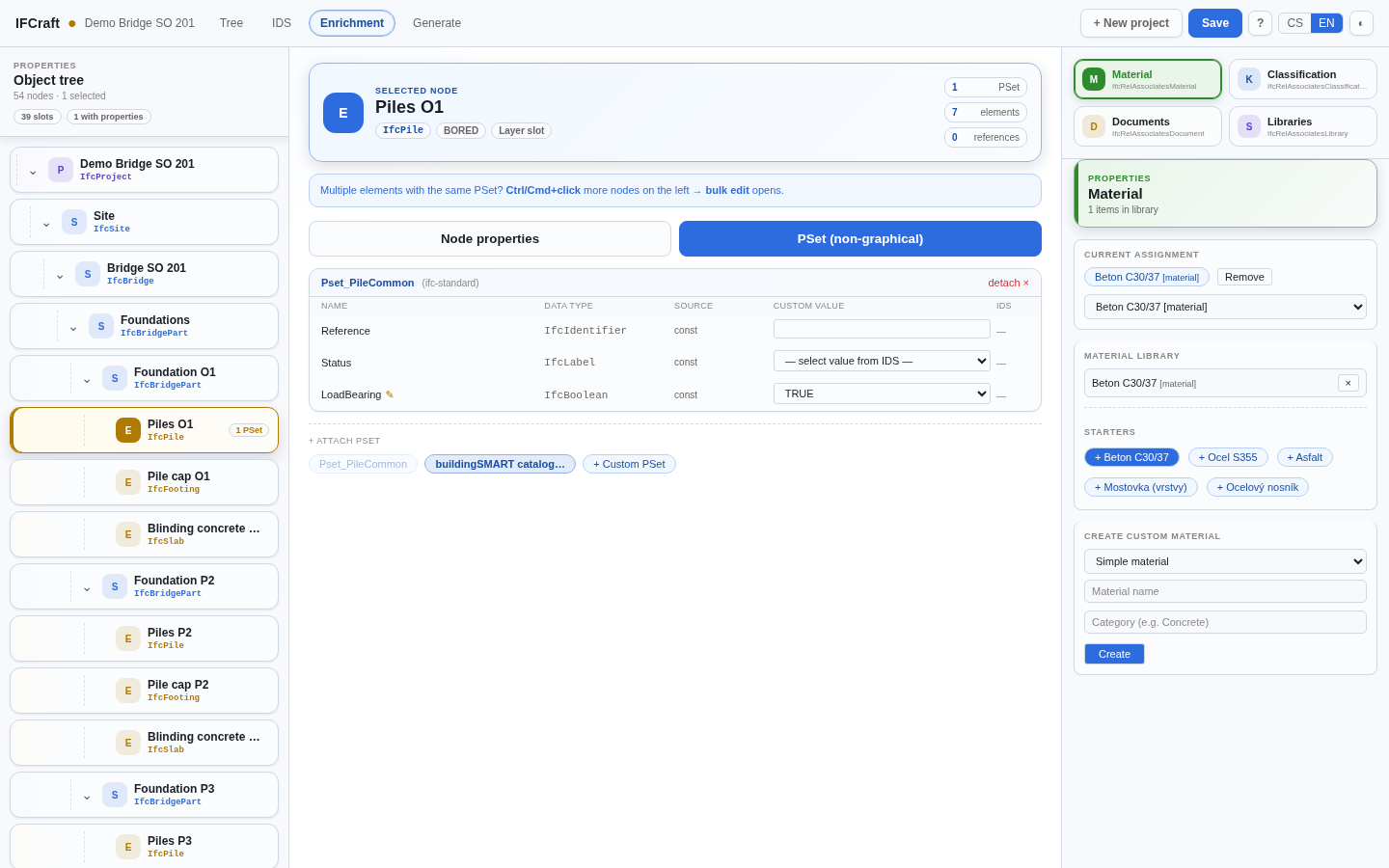
Classification. The Classification panel attaches a classification code (IfcClassification) to the element — for example from the SFDI data standard. Fill in System (IfcClassification.Name), Code (Identification), and Item name (Reference.Name). The "More IFC fields" section offers Source, Edition, URI, and other optional fields. If the node is bound to an IDS specification, the editor may suggest classifications found in that IDS.
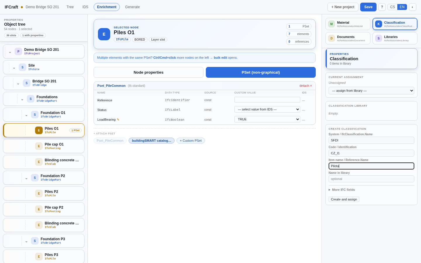
Documents and Libraries. The Documents panel (IfcDocumentInformation) and Libraries panel (IfcLibraryInformation) work the same way — they attach a reference to an external document (for example a technical report or drawing) or a reference library/standard to the element. Both associations work for one selected node at a time.
On the IDS tab you load the client's requirements in IDS format, assign individual specifications to tree nodes, and let them drive how the model is generated. IDS is therefore not just a checklist at the end — in IFCraft it feeds directly into the creation of the model.
IDS (Information Delivery Specification) is an open
buildingSMART standard in which the client (or a data standard, for
example SFDI) writes model requirements in machine-readable
form. Instead of a text appendix saying "for piles, state the
linear referencing method and classification", you receive an
.ids file that precisely states: for which elements
(applicability) which properties (requirements) apply, what data types
and formats they must have, and what values are permitted. The standard
workflow is to check the finished IFC against the IDS
afterwards — and then to track down and correct errors
laboriously.
IFCraft reverses this. IDS specifications are used immediately during model authoring: the required properties appear in PSets with pre-filled formats and locked enumerations, the export IFC class is governed by the entity requirement, and a final conformance check runs at export time. You deal with issues as you go, not over a finished file. It is the reverse of a BIM checker — instead of "check what was produced" you work in a "produce what should be produced" mode.
Upload an IDS file using the button next to the Load IDS
file: field (accepts .ids and .xml).
After uploading, an assignment filter and a table of specifications
appear.
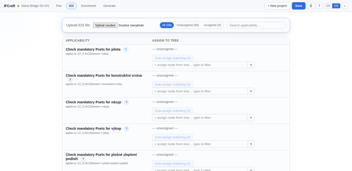
In the demo the file IDS_bridges_ifc_4x0.ids is loaded
with 56 specifications. The filter at the top shows
All (56) / Unassigned (56) / Assigned (0), and next to
it a Search applicability… field filters the table by
specification name (the search ignores accents and combines with the
active filter); the table has two columns:
Applicability (specification name and what it applies
to) and Assign to tree (a combo box for binding to a
node).
Each specification has two parts: applicability (which elements it applies to) and requirements (what they must satisfy). Click the ? button on a specification row to see both in an info window.
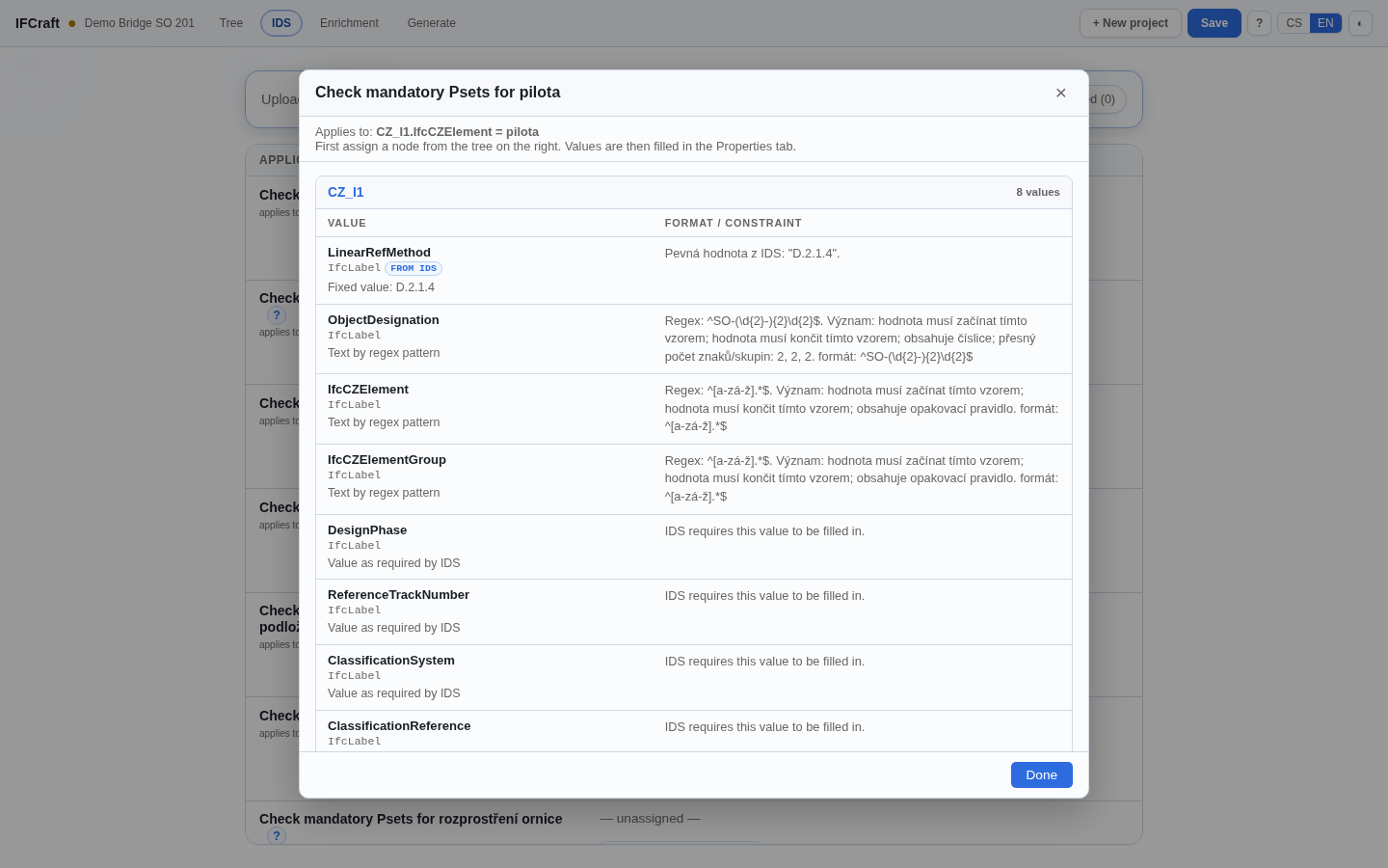
The window above shows the specification "Check mandatory Psets for pilota". At the top: Applies to: CZ_I1.IfcCZElement = pilota — this is applicability via the CZ_I1 classification. Below is a requirements table organised into PSets (CZ_I1, CZ_S2, CZ_S4, CZ_E1, CZ_M1, CZ_M3, CZ_F1, CZ_I8), each with columns Value and Format / constraint: LinearRefMethod has a fixed value "D.2.1.4." from IDS, ObjectDesignation expects text matching a regex pattern, and many properties simply require that a value is present ("IDS requires this value to be filled in."). The window only describes the requirements — values are filled in and validated on the Enrichment tab. Close it with the Done button.
For a specification to affect a specific element, you must assign it to a tree node. Each specification row has a combo box in the Assign to tree column; click the ▾ (Expand node selection) button to show the node list.
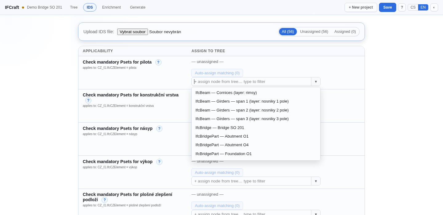
The list shows all 54 tree nodes, each with its IFC class and name. A
checkmark ✓ on a node would mean the node
matches the applicability of the specification (and
could be assigned automatically). In the demo no node has ✓ — and this
is instructive: the specification targets
CZ_I1.IfcCZElement = pilota, meaning elements with a
CZ_I1 classification, but the Demo Bridge project nodes
carry no CZ_I1 classification. The IDS applicability and the project
reality simply do not match — the function compares what the IDS
requires against what the nodes actually have. You can still assign the
specification manually: click a node to select it (in the demo the
"pilota" specification was manually assigned to
IfcPile — Piles O1).
After selecting a node, the combo box is replaced by a chip showing the assigned node (class, name, and layer), and the filter jumps to Unassigned (55) / Assigned (1). The chip can be removed with the × button.
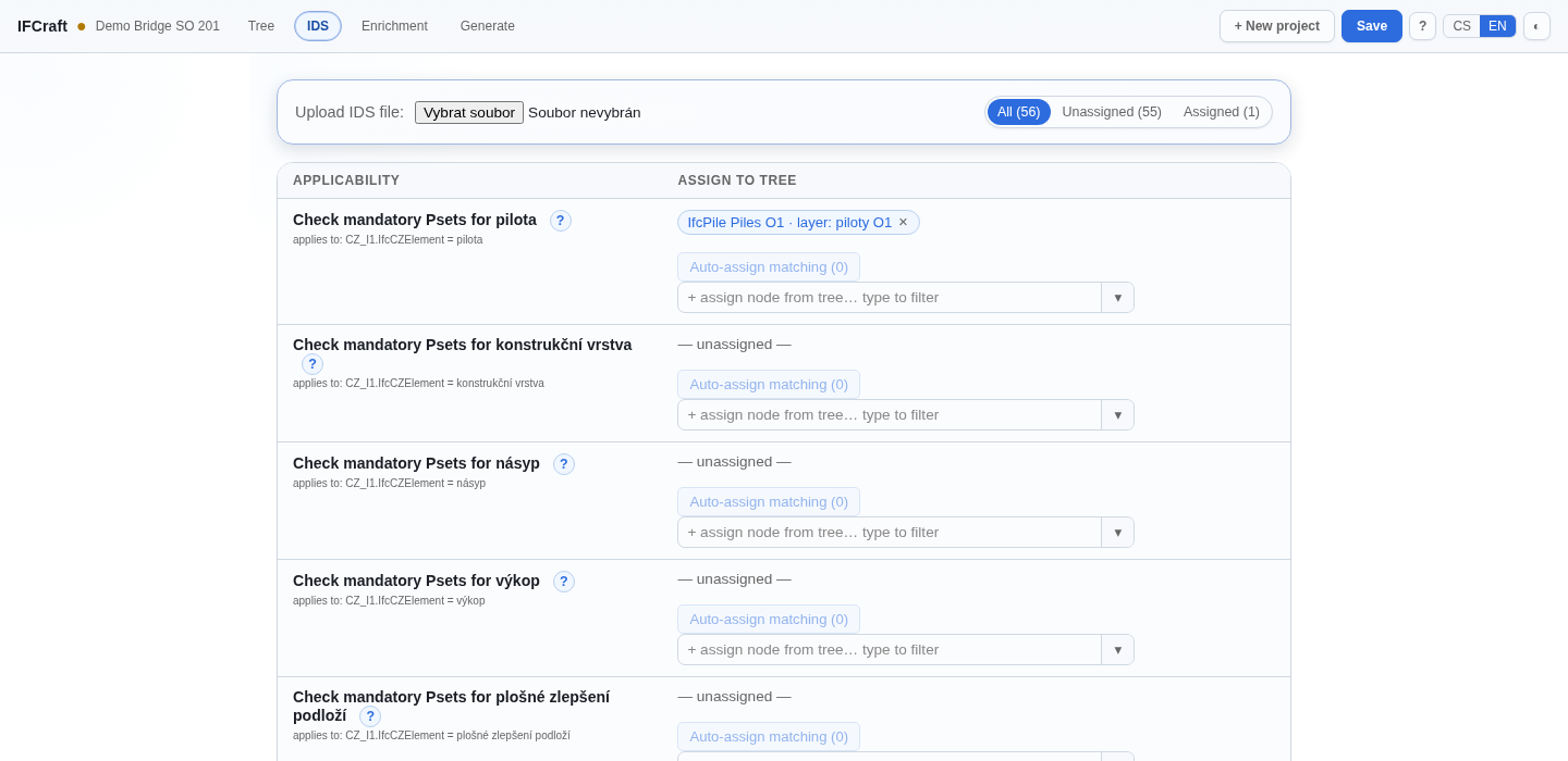
The Auto assign matching ({count}) button is always visible. When no tree node matches the specification's applicability (nodes lack the required classifications or properties), the button is greyed out with an explanatory tooltip and cannot be clicked. As soon as at least one matching node exists and is not yet assigned, the button shows the count and clicking it assigns all of them at once.
The filter above the table switches the view between all, unassigned, and assigned specifications — for 56 specifications this is a practical way to track what you have already bound.

Assigning a specification to a node is not just a label — it changes how the element is generated. The entity requirement from the IDS determines the export IFC class of the element (if the IDS prescribes a different class from the one the node has, the builder adjusts it when the IDS is bound and reports the changes in a "Changes to export classes from IDS" message). The required properties are also pre-filled into the node's PSets — with locked enumerations and prescribed formats.
You can see this by switching to the Enrichment tab → PSet
(non-graphical) for the assigned node. On
Piles O1, PSets scaffolded from the IDS (in the demo: CZ_I1
through CZ_I8 — eight PSets in total) appear with IDS
hints: fixed values are pre-filled (IfcCZElement = pilota,
LinearRefMethod = D.2.1.4), fields with a format constraint show the
validation message "Does not match the required format: …", and
enumeration properties offer only the permitted values. The
IDS column marks properties that the IDS requires.
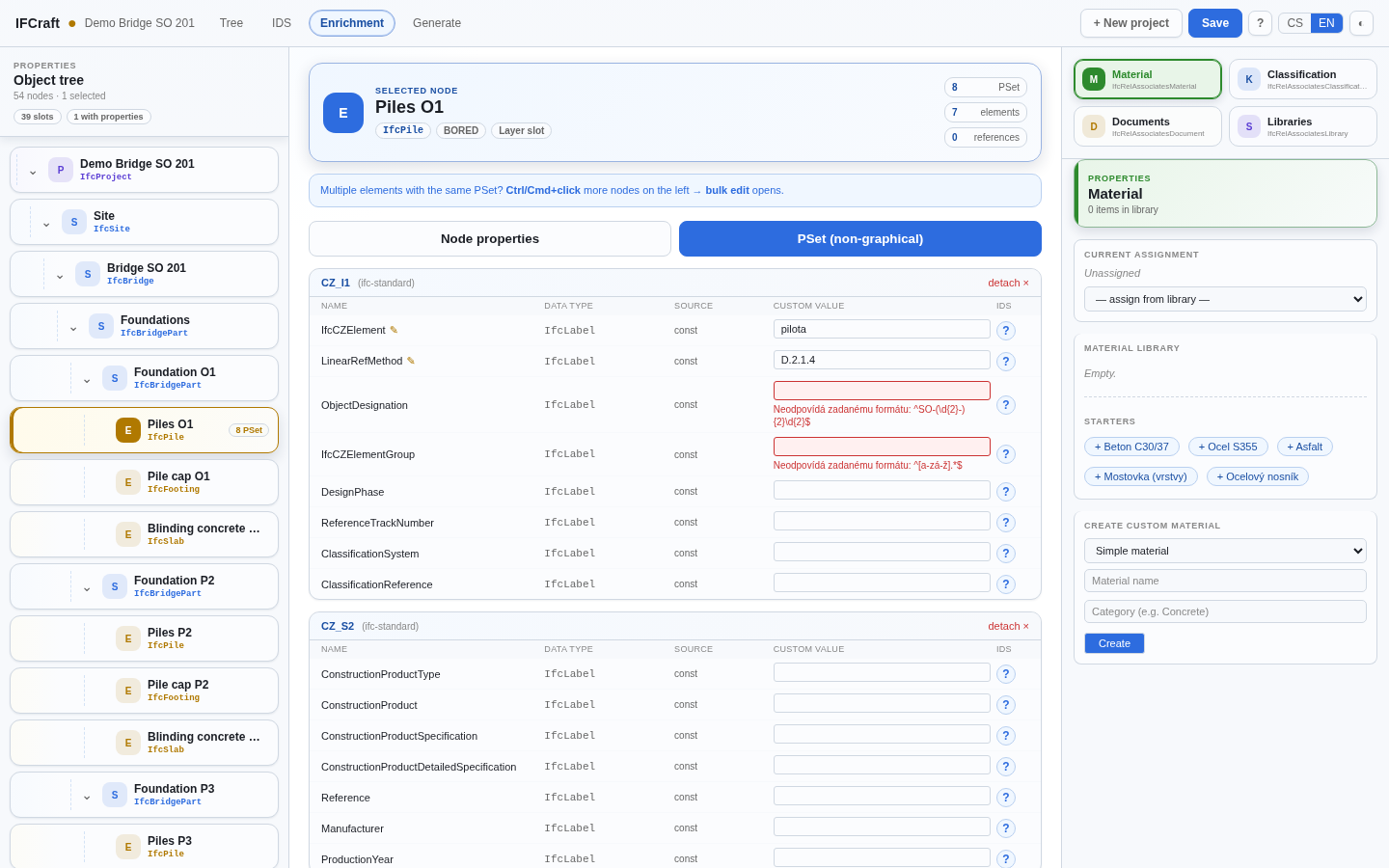
This way IDS guides the entire enrichment process: you know what needs to be filled in, right at the element, not only over a finished file. The final check — conformance of the generated IFC against the IDS — runs at export time; chapter 7 covers it in the section "IDS check".
The last tab — Generate — turns the finished Convention into an IFC file. Start with the project overview and fill in the metadata, then choose the output coordinates, run the build, and — if an IDS is loaded — pass the conformance check. Finally download the file and verify it in a viewer.
Download the finished IFC for the Demo Bridge: demo-bridge-so201.ifc
The Project overview card summarises in numbers what will be generated into IFC. It is a final sanity check that the Convention contains what it should.
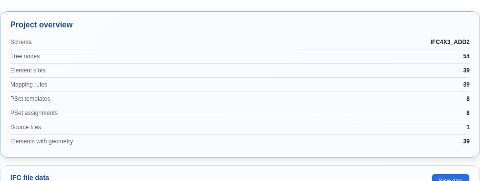
The rows mean:
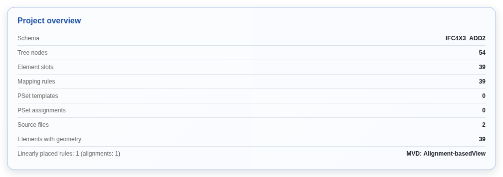
The Linearly placed rules: {N} (axes: {M}) — MVD: {label} row appears only when at least one rule uses linear placement along an axis. In the Demo Bridge project there are no alignments, so this row does not appear — the card ends at "Elements with geometry: 39".
The Output coordinates dropdown controls in which coordinate system the IFC is created. Two options are available:
The dropdown is shown only when the project has a local georeference ("local" mode, see chapter 11). The Demo Bridge SO 201 project was created without georeference, so the dropdown is not shown and the stats card ends directly at "Elements with geometry: 39" with no additional rows.
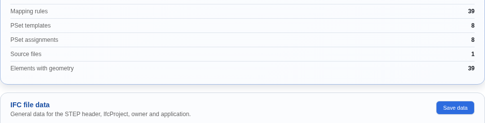
Georeference settings (which also make this dropdown available) are configured at project creation; chapter 11 covers them in detail.
The IFC file data form fills in general information
in the STEP header, in IfcProject, for the author, and for the
application. It is divided into sections File header,
IfcProject, Author, and
Application. Each field has a note on the right
indicating exactly where in the IFC the value is written (for example
FILE_NAME.author, IfcProject.Description).
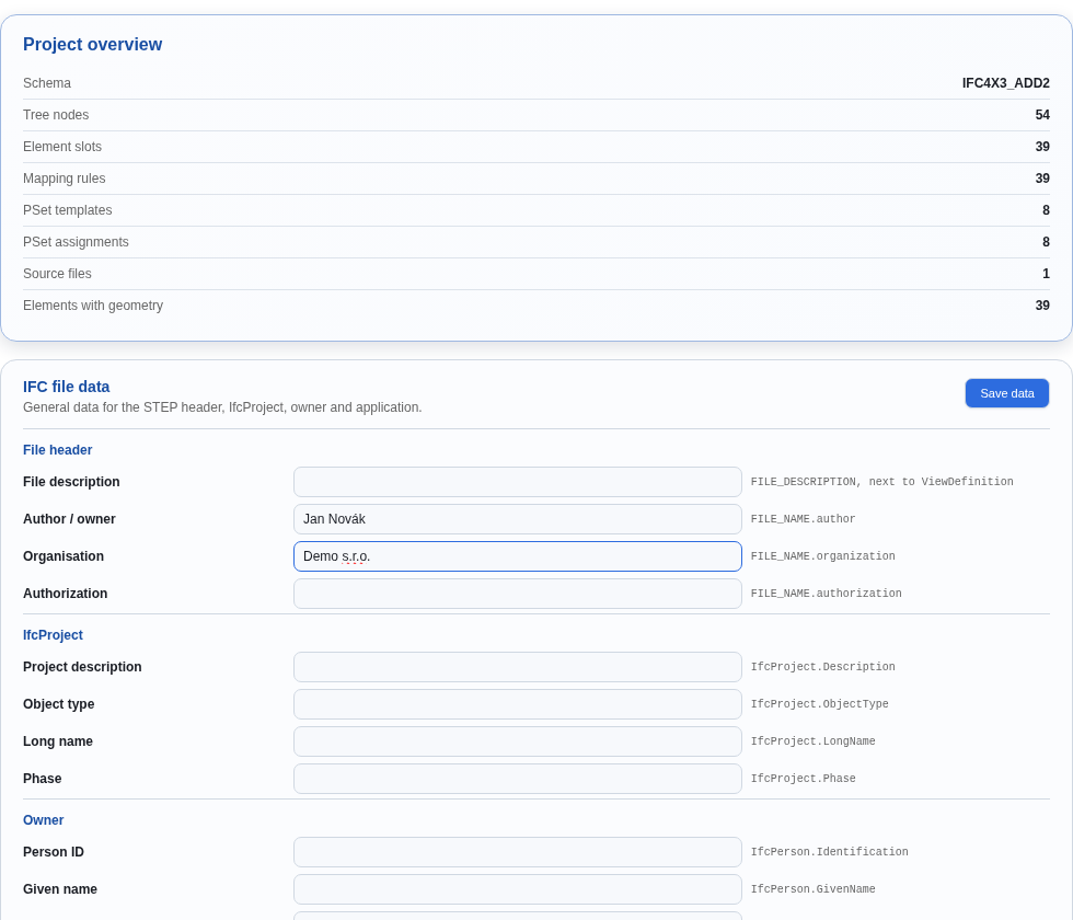
In the demo the Author field contains "Jan Novák" and Organisation "Demo s.r.o."; the Application fields are pre-filled (IFCraft). Save the filled-in data with the Save data button on the right — a confirmation "IFC data has been saved." appears and the data are written into the Convention, so they persist after reopening the project.
Before the file is generated, IFCraft may display build warnings. These checks do not block export, but signal that the result may not be what you expect:
A special case is geometry on a facility-part spatial element (IfcBridgePart, etc.). This is valid IFC, but non-standard according to the MVD. IFCraft therefore shows a permanent consent banner "⚠ Geometry on spatial elements … valid IFC but non-standard per MVD" and allows export only after checking "I acknowledge this and want to export anyway."
In the demo none of these warnings appeared — the project has no orphaned rules, no spatial nodes with layers, and no geometry on facility-parts, so neither the warning block nor the consent banner were rendered. No screenshot of this state is included; the only "gate" that appeared in the demo is the IDS check below — and the consent checkbox visible in figure 07-04 comes from that gate.
If an IDS is loaded in the project (chapter 6), IFCraft checks the conformance of the generated IFC against the IDS after building and shows the result as a gate:
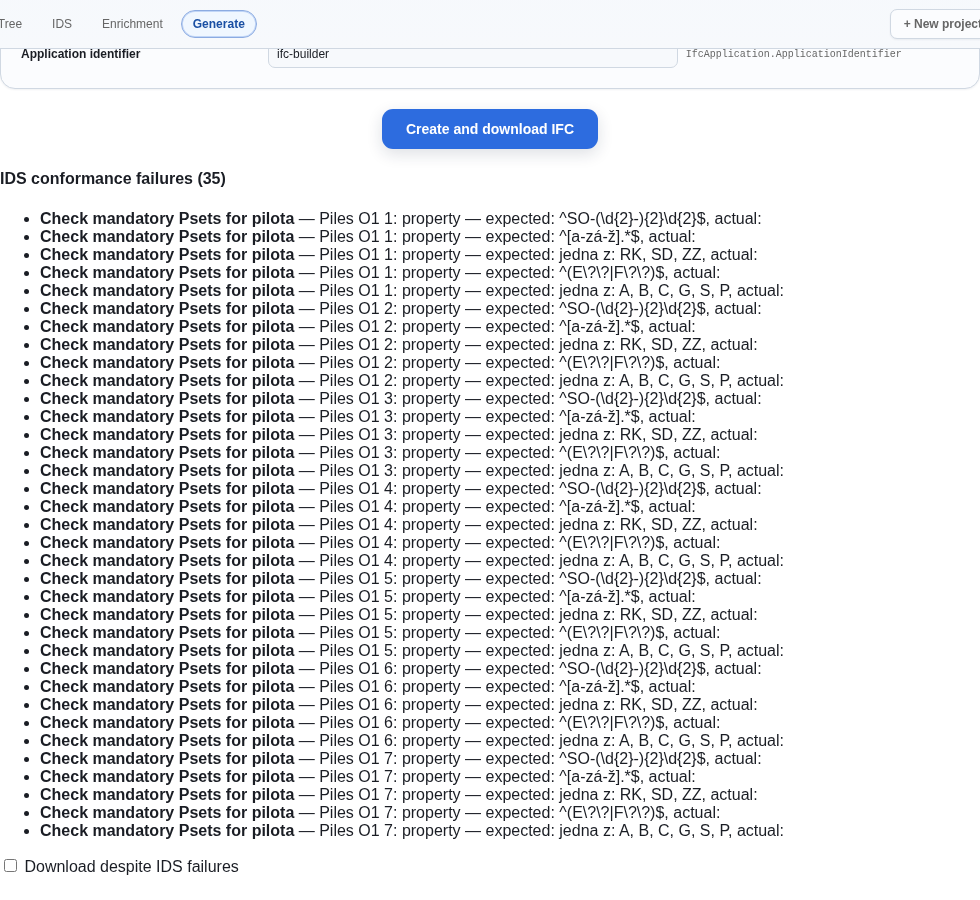
In the demo the gate is red with 35 non-conformances. They arise because the manually assigned specification "Check mandatory Psets for pilota" (chapter 6) has 5 scaffolded property requirements, and these are checked against 7 piles in the "Piles O1" node → 5 × 7 = 35 non-conformances (a regex/enumeration value is expected; the properties are actually empty). This is accurate information about the completeness of non-graphical data — not a defect of the STEP file; the generated IFC is still schema-valid.
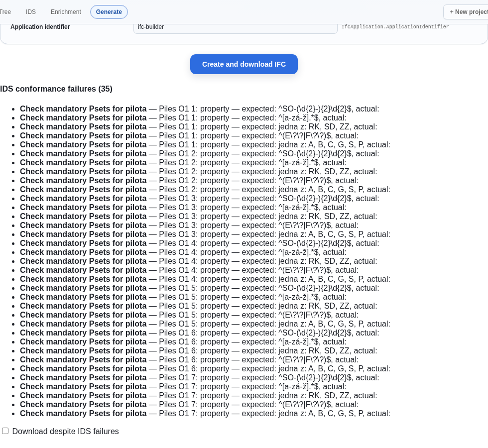
The blocked download can be deliberately unlocked by ticking "Download despite IDS non-conformances" at the bottom of the gate. This acknowledges that the model contains non-conformances and you are downloading it anyway.
Start generation with the Create and download IFC
button. The build runs in the browser (a few seconds for a large model).
If the IDS gate does not block the download (or you unlock it with the
consent), the file is downloaded and a STEP preview
appears below the button — the first 200 lines by default. Click
Show 500 more lines to load the next batch (up to a
limit of 10 000 lines); for the full content of a large file use the
downloaded file. Above the preview there is a search field: enter text
(for example IFCPROPERTYSET) and click Next
occurrence or press Enter — the preview scrolls to the first
match and automatically loads more lines if the match lies beyond what
is currently shown.
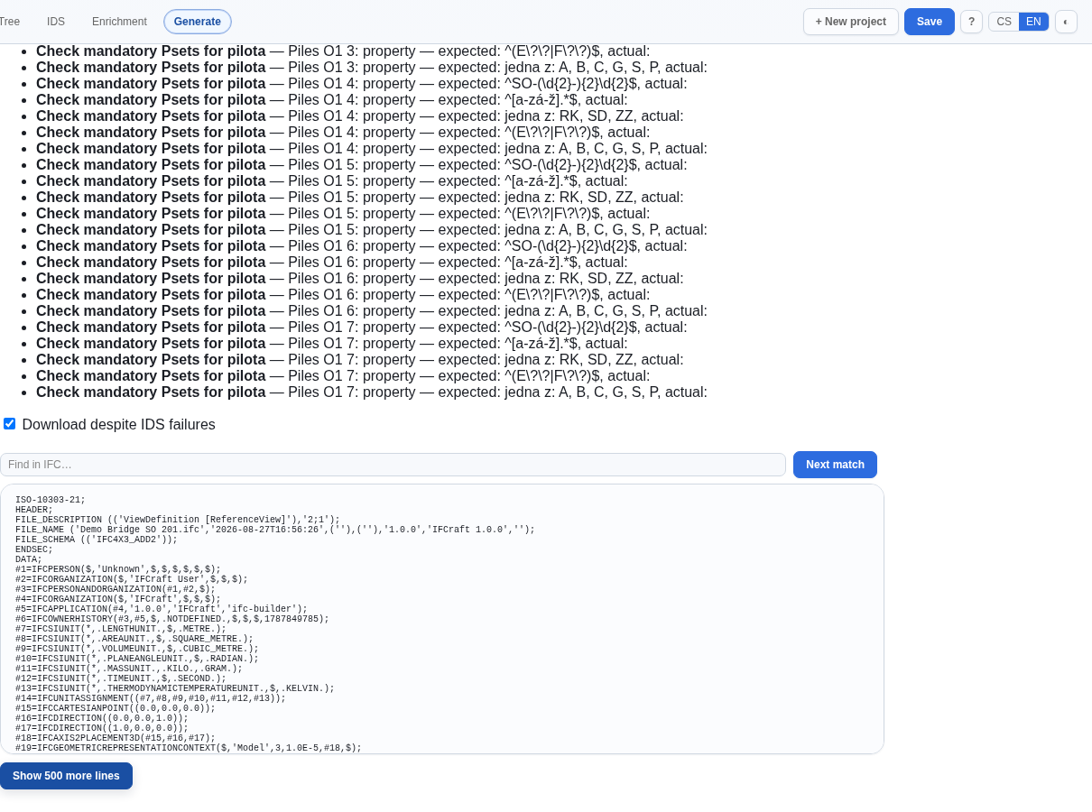
In the preview you can see the header: FILE_NAME with
author "Jan Novák" and organisation "Demo s.r.o.",
FILE_DESCRIPTION with
ViewDefinition [ReferenceView],
FILE_SCHEMA (('IFC4X3_ADD2')), and the beginning of the
data section (IfcPerson, IfcOrganization, IfcSIUnit…). The preview
confirms that the metadata and schema are correct.
Open the generated IFC in any IFC viewer and check that the geometry and structure loaded completely. The demo IFC was loaded in the online viewer IFC Navigator (web-ifc, no registration required, parsing runs locally in the browser).
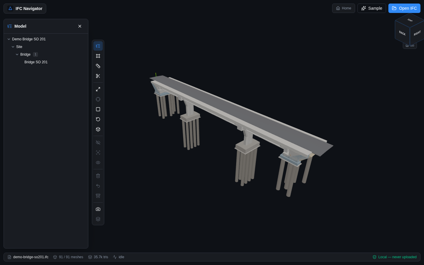
The viewer rendered the model completely (91/91 meshes) with the structure visible in the left-hand tree (Demo Bridge SO 201 → Site → Bridge). You can see the pile groups, pile caps, piers, abutments, and the deck with the surface course — exactly what was in the Convention.
In addition to a visual check, we recommend validating the file:
For a clean pass of the "Industry Practices" rules of the online validator too, the demo carries georeferencing (chapter 11 — rule GRF003 expects a coordinate reference system in a model with IfcBridge) and exports the piles as mesh (see the IFC430 note in chapter 5).
Validation confirms that the file is technically correct; the IDS gate (above) is a different check — it monitors the completeness of data according to the client's requirements, not the correctness of the STEP file.
Sometimes one physical element is made of several materially distinct parts that live on separate layers in the source model. A beam is concrete plus reinforcement, a bridge deck is the load-bearing slab plus crossbeams, a layered structure has a base course and a wearing course. IFCraft can describe such an element as one IFC product with named parts — instead of splitting it into independent elements, it creates a single element whose geometry is internally structured and whose parts can carry different materials and colours.
Two panels you already know meet here: layers are bound in the Tree (chapter 3), pairing and granularity live in Enrichment (chapter 5).
Create a composite element when both conditions hold:
deska_pricniky — the deck with crossbeams — and
rimsy — the cornices).If it is fine for each layer to become its own element, you do not need a composite — give each layer its own node, as the Demo Bridge Convention does everywhere else. A composite makes sense where the parts belong together semantically and should behave as one object with internal structure in the IFC.
Select an element node in the Tree — in the demo Deck with
crossbeams (IfcSlab, layer deska_pricniky). Its
detail panel has the Geometry and layer section with
one BOUND LAYER block. The element becomes composite
the moment you add a second block: pick another layer in the Add
layer dropdown at the bottom — in the demo rimsy —
and a second block appears.
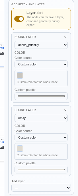
Each block has:
Add blocks until all parts of the element are covered. Deleting a block removes the part; deleting the last block frees the slot (the node stops being composite and the layer is unbound).
In the demo both parts were given a Custom color
from the project palette: #c9c6c0 for the deck part and
#e0dcd3 for the cornices, so each part is distinguishable
in a viewer.
When a node has more than one layer, additional settings appear in Enrichment (the Node properties tab). They control how many elements are produced and how objects from the different layers are paired into one element.
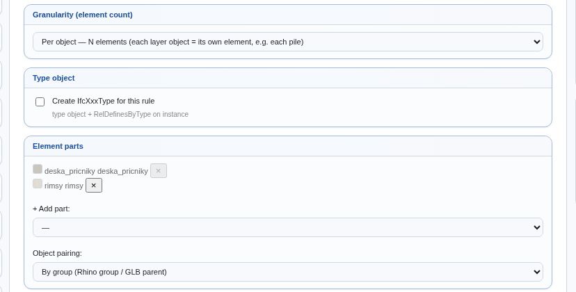
Granularity (element count) decides whether the layers produce one element or several:
Element parts lists the individual parts (each
bound layer) with their colour swatches and lets you manage them from
here too (+ Add part:, remove with ×).
Object pairing determines how objects from different layers are matched into one group (shown for the Per object granularity):
groupKey). This
is the right choice when the source model records which parts belong
together.The demo file has no Rhino groups on these layers (8
deck objects, 2 cornice objects, no groupKey), so By group
has nothing to match on and the deck is one continuous structure anyway
— the demo therefore uses Aggregate, which produces a
single composite product.
From a composite element IFCraft generates one IFC product with internally structured geometry:
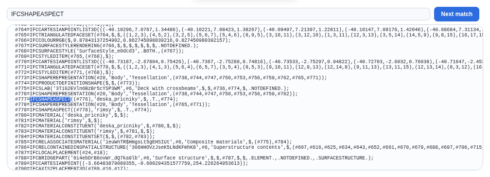
The preview shows the real output of the demo: a single
IFCSLAB('Deck with crossbeams') whose shape is split into
two IFCSHAPEREPRESENTATIONs, one
IFCSHAPEASPECT named deska_pricniky and one
named rimsy, followed by
IFCMATERIALCONSTITUENT entities for both parts, the
IFCMATERIALCONSTITUENTSET, and the
IFCRELASSOCIATESMATERIAL that attaches "Composite
materials" to the product. The two IFCSURFACESTYLE entities
above carry the custom part colours (SurfaceStyle_c9c6c0,
SurfaceStyle_e0dcd3).
Schema difference:
IfcMaterialConstituentSetexists only from IFC4 onwards. When exporting to IFC2x3 the material set is omitted, butIfcShapeAspect(the named geometry parts) remains — the parts stay geometrically distinguishable in IFC2x3, just without the material set. See chapter 12 for schema differences.
Composite elements can also be placed linearly along an alignment (chapter 10).
An assembly (IFC class IfcElementAssembly) is the opposite principle to the composite element from chapter 8. While a composite is one product with internally structured geometry, an assembly is a group of standalone elements that belong together but remain individually addressable in the model. Typical examples: a steel structure made of beams and plates, a precast segment composed of several units, or — as in the demo — a pier composed of its stem and bearing plinths.
Use an assembly when you want to preserve the relationship "these elements form one erection unit", but each unit must remain a separate element with its own geometry, material, and properties.
An assembly is a node of class IfcElementAssembly
with element children (the individual units). The
assembly node itself carries no geometry — its children do. In the IFC,
the link between the assembly and its units is written as a
decomposition (IfcRelAggregates), not as
spatial containment. That is the essential difference: the units are not
"located in" the assembly as in a space; they are its
components — the assembly is built from them and can be
taken apart again.
Create the assembly in the Tree: select the parent node and add a node of class IfcElementAssembly from the palette (it is offered among the element classes under any spatial part). Then add the element children under the assembly node — the palette on an assembly offers the element classes, so you build its units exactly like any other element slots and bind their layers.
In the demo the bridge part Pier P2 contains an
assembly named Pier P2 assembly with two element
children taken from the original Convention: Pier stem
P2 (IfcColumn, layer drik P2) and Bearing
plinths P2 (IfcFooting, layer
podloziskove bloky P2, granularity Per object).
When you select the assembly in Enrichment (the Node properties tab), an Assembly card appears with a granularity choice:
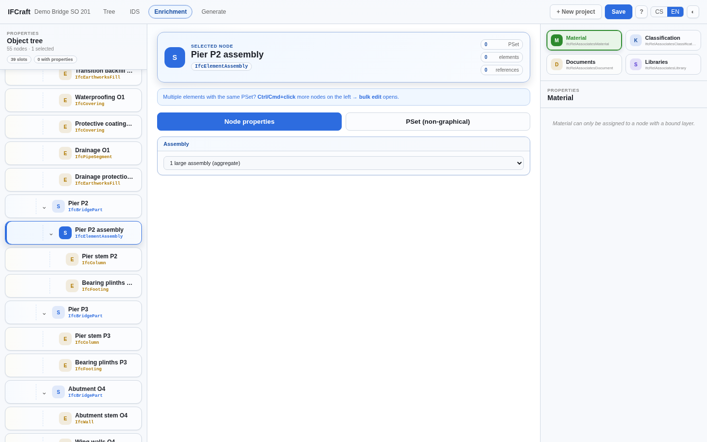
The granularity has two options:
groupKey — Rhino group / GLB parent). Each group
yields one assembly with its own units. Use this when the same erection
unit repeats in the model (for example, every bridge span = one
assembly).Assemblies share the group-pairing mechanism (groupKey)
with composite elements from chapter 8 — the instance granularity needs
source data with groups to know which units belong to which assembly.
The demo file has no groups, so the demo keeps the default 1
large assembly (aggregate).
If, with the instance granularity, a group is incomplete (a unit expected from one of the layers is missing in the source), IFCraft still creates the assembly from the available children and adds a warning — it does not silently drop the incomplete assembly.
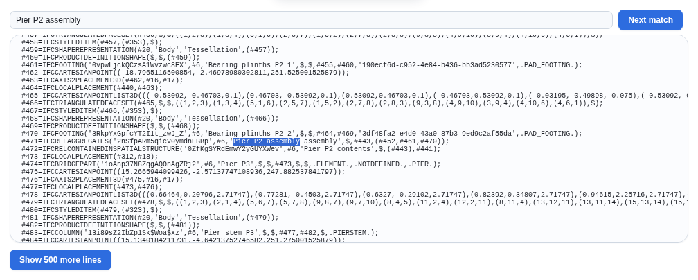
From the assembly node the demo produces exactly the structure visible in the preview:
IFCELEMENTASSEMBLY('Pier P2 assembly'), without geometry of
its own.IFCCOLUMN (the pier stem) and two IFCFOOTINGs
(the bearing plinths — their slot uses Per object granularity, so each
plinth is its own element).Note on the demo state: the screenshots come from a prepared project state in which the two existing element slots of Pier P2 were nested under a new IfcElementAssembly node. Building the same structure by hand — palette: add IfcElementAssembly, then add the element slots under it and bind their layers — produces the identical result.
Linear referencing places an element in the model by station along an alignment instead of by absolute coordinates. For linear structures (roads, railways, bridges) this is the project's natural language: a pier is not "at X=…, Y=…" but "at station 1+078, half a metre right of the axis". IFCraft supports this logic — elements can be bound to an alignment from LandXML and their position is written into the IFC linearly.
Linear placement is an IFC4x3 feature (the infrastructure schema). IFC2x3 and IFC4 have no entities for linear placement — choose IFC4x3 for linear structures.
When an element is placed linearly, its position is tied to the alignment: it is defined by the station (position along the axis) and offsets (lateral left/right and vertical). This has two big advantages:
The alignment enters the project as a LandXML source
file (chapter 4 — + Add file in the Tree).
LandXML carries only the axis geometry (horizontal + vertical profile
and stationing), no mesh — it is purely a route definition. In the demo
we add demo-axis.xml, a 200 m straight axis running along
the bridge with stationing starting at 1+000.
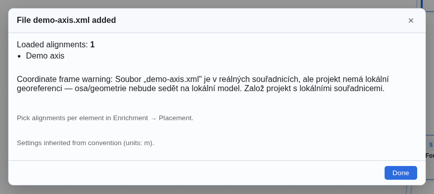
The modal reports Loaded alignments: 1 ("Demo axis") and shows a coordinate frame warning: LandXML files are treated as real-world coordinates, and the Demo Bridge project was created without georeference, so IFCraft cannot verify that the axis and the model share a frame. It warns that the axis may not sit on the local model. In the demo the axis was authored in the same coordinate range as the model, so the projected values below come out sensible — but read this warning seriously with real data: if the axis lies hundreds of kilometres from the model, stations and offsets will be nonsense. The clean solution is a project with a local georeference (chapter 11).
The file then appears in SOURCE FILES as
demo-axis.xml — landxml · 1/1 alignments. Clicking the
alignments count opens a picker where individual axes of a
multi-alignment file can be enabled or disabled.
Linear placement is configured in Enrichment on an element node, in the Placement card. Switch the radio from Absolute (coordinates) to Linear (along alignment) and pick the axis in the Alignment dropdown. In the demo we place the Pavement element (IfcPavement, the surface course — a natural candidate for stationing along the route).
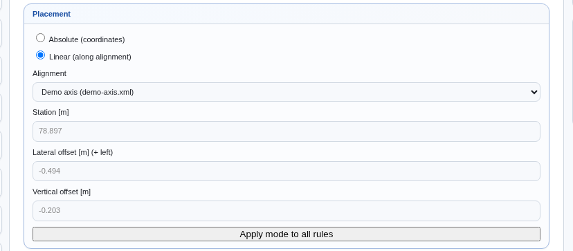
After you select the alignment, IFCraft automatically computes the projection of the element onto the axis and pre-fills the placeholders:
The values are placeholders — the auto-projection from the element geometry and the axis. You can keep them or type your own. The Apply mode to all rules button sets the same placement mode on all rules at once.
Note that the station field shows the distance along the axis
geometry; the axis itself starts at station 1+000 (staStart
in the LandXML), so the resulting station written into the IFC is
1+078.897.
On the Generate tab, the project overview now shows the row Linearly placed rules: 1 (alignments: 1) and the MVD switches to Alignment-basedView:
From a linearly placed element IFCraft generates:
Viewers and CDEs, however, usually do not display
the values of the placement itself (station, offsets). IFCraft therefore
additionally emits the PSet
IFCB_LinearPlacement — a readable list of the
placement parameters directly as element properties:
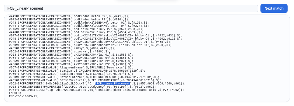
In the demo output the PSet contains AlignmentName =
"Demo axis", Station = 1078.897, StationFormat
= "1+078.897", OffsetLateral = −0.494 (slightly right of
the axis), and OffsetVertical = −0.203. These values appear
in any viewer as ordinary element properties, so the engineer sees the
station even when the viewer does not interpret
IfcLinearPlacement itself. Below the PSet you can see the
IFCRELPOSITIONS relation tying the Pavement product to the
Demo axis.
Linear placement on composite elements. Linear placement also works on composite elements (multiple layers, chapter 8). The composite is placed as a whole — the anchor is the centroid of all its parts and each part keeps its relative position. With the Per object granularity each group of objects gets its own station (derived from the group's position along the axis); with Aggregate a single linear placement is created for the merged element.
Besides placing elements on the axis, IFCraft can also emit station points — standalone reference points on the alignment. In the IFC they become IfcReferent entities with the standard Pset_Stationing property set. They mark significant stations on the route (start/end of a structure, principal points). Unlike linearly placed elements, referents do not count towards the Alignment-basedView MVD decision.
Georeferencing says where in the world the model lies — in which coordinate reference system and at what position. For infrastructure this is essential: without a georeference the model cannot be set out on site or reliably combined with surrounding data (terrain models, utilities, neighbouring structures). IFCraft handles georeferencing in two places — when the project is created (where the coordinates come from) and at export (in which coordinates the IFC is written).
This chapter covers both and builds on chapter 2 (Creating a project) and chapter 7 (Generate), where the same controls appear in context.
The coordinate system is set on the start screen when creating a project, in section 2 · Location and coordinate system. You choose one of three modes:
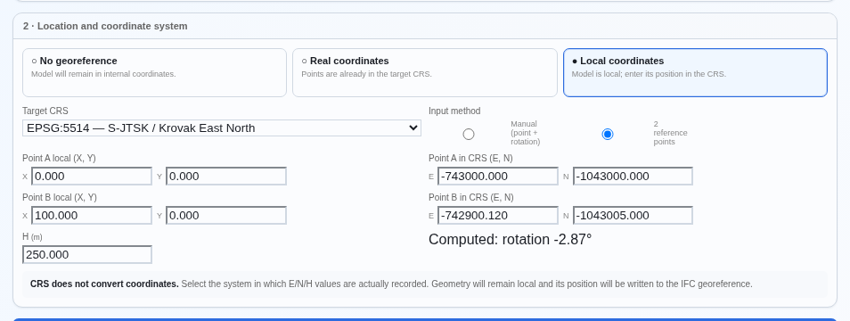
For the real and local modes you pick the Target CRS. IFCraft offers presets for the most common systems:
The CRS does not convert coordinates. The choice only records which system the entered values are held in — it does not transform the geometry between systems. Select the system in which the model coordinates (or the origin position) are actually recorded.
Mind the signs with EPSG:5514. Krovak East North has negative E and N (E = −Y, N = −X of classic S-JTSK). Positive values are most likely classic Y/X — enter them with a minus sign, otherwise LandXML alignments will not match the model. IFCraft shows a warning when positive values are entered for this CRS.
In the local mode you enter the position of the local origin (E/N/H) and how the rotation is determined. The Input method toggle offers two methods:
You enter two points known in both systems — local and real. The application computes the rotation from them and shows it as "Computed: rotation X°" (in the demo figure −2.87°). If the distances between the points differ by more than 0.1 % between the local and the real system, a warning appears — check the entered coordinates.
Use this method when you have surveyed points with known coordinates in both systems.
You enter one reference point (the position of the local origin in the CRS) and the rotation in degrees directly. Use it when you know the model's rotation from elsewhere — the design documentation or the axis azimuth.
There is no scale input. The model is assumed to be
in a local survey network where
IfcMapConversion.Scale = 1 holds.
Surveyors working in a local network already convert coordinates into
it, so a separate scale parameter is not needed.
The second place where the georeference matters is Generate — the Output coordinates dropdown at the bottom of the project overview card. It controls in which coordinates the IFC is actually written:

The dropdown appears only when the project has a local georeference. For projects created without georeference (like the demo in chapters 2–10) it is not shown — an informational row takes its place (chapter 7).
For a project with a local georeference (EPSG:5514, origin E −743 000 / N −1 043 000 / H 250, rotation −2.87° — the values from the form above), the generated file contains:
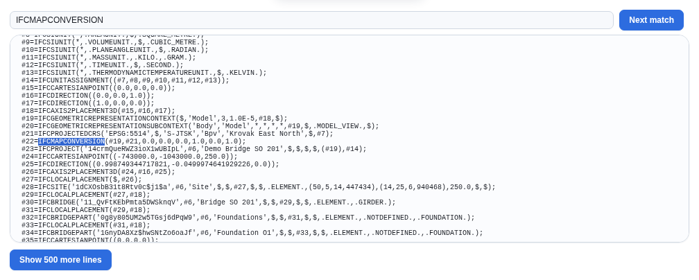
'EPSG:5514' with the
S-JTSK / Bpv description.Note on the demo state: the Demo Bridge project itself was created without georeference; for the figures above, a copy of the finished demo Convention was given the local georeference corresponding to the form in figure 11-01. Creating the project with Local coordinates from the start leads to the same output. The downloadable demo IFC (chapter 1) corresponds to exactly this georeferenced state.
The entities carrying the georeference — IfcMapConversion and IfcProjectedCRS — exist only from IFC4 onwards. When exporting to IFC2x3 they are not emitted: the georeference settings stay stored in the project but are not written into the IFC2x3 file. For georeferenced output choose IFC4 or IFC4x3. See chapter 12 for the schema overview.
This chapter is a reference — it summarises what each input format brings into IFCraft, how the target IFC schemas differ, which IFC classes the demo Convention uses, and how to solve the most common problems. Come back to it whenever you need to check something quickly.
IFCraft reads six input formats. Each contributes differently — some carry layers and geometry, LandXML only alignments. The table summarises what each format actually yields (verified from the source extractors):
| Format | Layers | Groups (groupKey) |
Colours | UserStrings / attributes | Alignments |
|---|---|---|---|---|---|
| 3DM (Rhino) | yes — Rhino layers (fullPath) | yes — Rhino groups | object + layer | yes — read into attributes | no |
| DXF (AutoCAD) | yes — LAYER table | yes — ACAD_GROUP | yes — ACI palette (object + layer) | no | no |
| DWG (AutoCAD) | yes — LAYER table | yes — ACAD_GROUP | yes — ACI palette (object + layer) | no | no |
| GLB (glTF 2.0) | yes — node/mesh name | yes — parent node | object only — material (baseColor) | no | no |
| OBJ (Wavefront) | yes — g/o groups |
no | no | no | no |
| LandXML | — (no mesh) | — | — | — | yes — H+V alignments only |
Details per format:
fullPath, i.e. the full path of nested layers). Groups are
read from the Rhino group table (groupKey = group name), so
3DM is a good source for composite elements and assemblies with the
instance granularity. Colour is taken from the object (object colour)
with a fallback to the layer colour. Object UserStrings are read into
object attributes and can be mapped to PSet properties via the "From
model (UserString)" source in the custom PSet editor (chapter 5).256 means ByLayer, 0 ByBlock.
Geometric entities read: 3DFACE, SOLID, CIRCLE, LWPOLYLINE,
POLYLINE, MESH (closed polylines and circles are tessellated)
and 3DSOLID — ACIS bodies are converted to meshes
without a CAD kernel (planar, analytic and NURBS surfaces including
trimmed ones; solids with no stored ACIS data cannot be converted, see
Troubleshooting). Groups are read from the ACAD_GROUP
dictionary (groupKey = group name).groupKey). Colour
comes from the material (baseColorFactor) — object level
only, no layer colours. The geometry is already tessellated.g/o
groups become layers (the last, most specific name
token is used); several objects in one group yield several objects of
the same layer. OBJ carries no groupKey
(its groups are the layers themselves) and no colours — the geometry is
a plain mesh.IFCraft exports to three schemas. They differ in the available entities — the table summarises what matters:
| Feature | IFC2x3 | IFC4 | IFC4x3 |
|---|---|---|---|
| Mesh geometry | IfcFacetedBrep (closed) / SurfaceModel (open) | Tessellation | Tessellation |
| Georeference (MapConversion / ProjectedCRS) | no | yes | yes |
| Part materials (IfcMaterialConstituentSet) | no (ShapeAspect remains) | yes | yes |
| Quantities (IfcElementQuantity / Qto sets) | no | yes | yes |
| Infrastructure entities (IfcBridge, IfcRoad…) | no | no | yes |
| Alignment (IfcAlignment) | no | no | yes |
| Linear placement (IfcLinearPlacement) | no | no | yes |
| MVD (Model View Definition) | CoordinationView_V2.0 | ReferenceView_V1.2 | ReferenceView / Alignment-basedView* |
* With IFC4x3 the MVD switches to Alignment-basedView only when at least one linear placement is actually emitted on a product (chapter 10); otherwise it stays ReferenceView.
Practical consequences:
The Convention of chapters 2–7 uses the following classes — a practical starter set for a road bridge:
| Class | PredefinedType(s) in the demo | Used for |
|---|---|---|
| IfcBridge | GIRDER | the bridge as a whole |
| IfcBridgePart | FOUNDATION, SUBSTRUCTURE, ABUTMENT, PIER, SUPERSTRUCTURE, SURFACESTRUCTURE | the spatial breakdown (per support) |
| IfcPile | BORED | bored piles |
| IfcFooting | PILE_CAP, PAD_FOOTING | pile caps, bearing plinths |
| IfcSlab | BASESLAB, APPROACH_SLAB, (none) | blinding concrete, approach slab, deck |
| IfcWall | SOLIDWALL, RETAININGWALL | abutment stems, wing walls |
| IfcColumn | PIERSTEM | pier stems |
| IfcBeam | BEAM, CORNICE | girders, cornices |
| IfcCovering | MEMBRANE, (none) | waterproofing, protective coating |
| IfcPipeSegment | RIGIDSEGMENT | drainage |
| IfcEarthworksFill | TRANSITIONSECTION, BACKFILL | transition backfill, drainage protection |
| IfcPavement | FLEXIBLE | the surface course |
| IfcElementAssembly | — | assemblies (chapter 9) |
The palette in the Tree offers the full IFC4x3 class set (about 150
element classes); the table lists what the demo actually uses.
(none) means the PredefinedType is left unset.
| Shortcut | Where | Action |
|---|---|---|
| Ctrl/Cmd+S | everywhere | Save the project |
| Ctrl/Cmd+click | Tree, Enrichment | Multi-select nodes (bulk edit) |
| Delete | Tree | Delete the selected nodes |
| Ctrl+Shift+R | browser | Hard reload (see Troubleshooting) |
Some 3DSOLID bodies from DXF/DWG have no geometry.
3DSOLID bodies are converted automatically, but only when the file
actually stores their ACIS data. After loading, the app reports how many
solids were recovered (e.g. "3D solids (ACIS): 101/101 fully recovered")
— a lower number means solids without stored data or with exotic surface
types. Solution: convert those solids to meshes in
AutoCAD with the _MESHSMOOTH command and save, or export
3DM (Rhino).
The LandXML alignment is far from the model. When the imported axis is in a different (real-world) coordinate system than the local model, the positions do not match. IFCraft detects this and shows a coordinate frame warning in the import modal — "the file is in real coordinates but the project has no local georeference" (chapters 4 and 10). Solution: either create the project with the corresponding local georeference, or use an axis in the same frame as the model.
Elements without geometry in the output. When an element slot has a rule but the layer has no mesh (or the slot has no layer bound at all), the element is created without geometry. IFCraft warns about this at build time on the Generate tab — "IFC will have no geometry", or orphaned rules (chapter 7). Solution: check the layer bindings in the Tree.
The "geometry on a spatial element" banner. If geometry ended up on a facility-part spatial node (IfcBridgePart etc.), it is valid IFC but non-standard per the MVD. IFCraft shows a permanent consent banner and allows the export only after you acknowledge it (chapter 7).
"The screen failed to load". If this message appears with an error description instead of a screen, the usual cause is a stale cache after an application update. Solution: hard-reload the browser — Ctrl+Shift+R.
The PSet catalogue in the "PSet (non-graphical)" tab is generated
from the official Property Set Definition (PSD) files
of the buildingSMART International IFC specification. The files cover
the IFC2X3, IFC4, and IFC4X3 schemas (281 / 451 / 690 templates). The
catalogue is regenerated with npm run gen-psets (script
scripts/gen-psets.py) and stored in
data/ifc-schemas/psets.<schema>.json.